OSA Lab · User manual
Control and logging of bench instruments over GPIB, USB, LAN and RS-232, all in one window.
1. What OSA Lab is
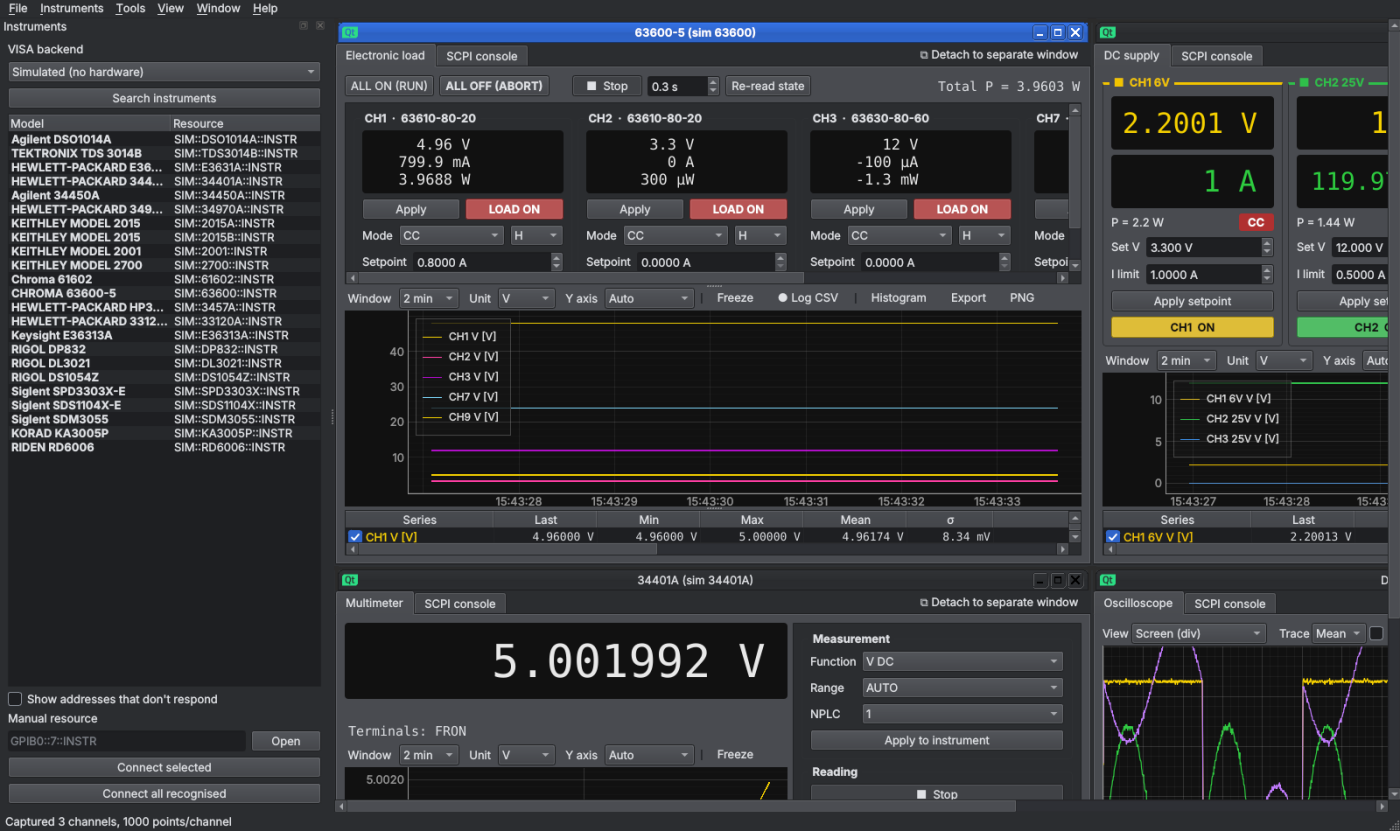
OSA Lab brings your bench instruments into a single program: power supplies, multimeters, oscilloscopes, electronic loads, AC sources, generators and data-acquisition units. Each instrument opens in its own window inside a workspace, which you can spread over several monitors and save.
- Live readings with a plot, statistics and CSV logging.
- Full control: setpoints, outputs, ranges, oscilloscope scales…
- A readings panel with big tiles to see everything at a glance.
- A combined log that puts readings from several instruments into one CSV.
- A sequencer to automate tests (load steps, holds, safety limits).
- A simulated mode to try everything without hardware.
2. Supported instruments
| Type | Models | Usual interface |
|---|---|---|
| Oscilloscope | Agilent/Keysight DSO1000A/B (DSO1012A, 1014A, 1024A…), InfiniiVision 5000/6000/7000 and 1000X–4000X (DSOX/MSOX/EDUX); Tektronix TDS3000 (TDS3014B…), MSO/DPO/MDO 2000–4000, MSO 4/5/6 Series, TBS1000/2000 | USB, GPIB, LAN |
| Multimeter | Agilent 34401A, 34405A, 34410A/11A, 34450A, 34460A/61A/65A/70A; Keithley 2000, 2001, 2002, 2010, 2015 THD, 2016, DMM6500, DMM7510; HP 3457A; Fluke 8808A; Keysight EDU34450A; R&S HMC8012; Aim-TTi 1906/1908 | GPIB, USB, RS-232 |
| DC supply | Agilent E3631A; E3640A–E3645A; HP/Agilent 6611C–6614C, 6631B–6634B, 6641A–6655A, 6671A–6675A; Keysight E36311A, E36312A, E36313A, EDU36311A; GW Instek GPD-2303S/3303S/4303S and GPP-1326/2323/3323/4323; BK Precision 9100/9200; Owon SPE and P4000; R&S HMC8041/8042/8043 and NGE100; Aim-TTi CPX400, QPX600/1200, MX100/180, PL/PLH | GPIB, RS-232, USB, LAN |
| Source-measure unit (SMU) | Keithley 2400/2401/2410/2420/2425/2430/2440 and 2450/2460/2461/2470; Keysight B2901A/B2902A/B2911A/B2912A | GPIB, USB, LAN |
| Data acquisition | Agilent 34970A (34901A/02A/03A/07A… cards); Keithley 2700 (7700/7702/7708… cards and front DMM); Keithley DAQ6510 (SCPI mode) | GPIB, RS-232 |
| Electronic load | Chroma 63600 (63610-80-20, 63630-80-60, 63640-80-80…); Siglent SDL1020X/1030X; BK Precision 8500B/8600 | GPIB, USB, LAN |
| AC source | Chroma 61600 (61601…61605) | GPIB, USB |
| Generator | Agilent 33120A, 33210A, 33220A, 33250A; Keysight 33500B, 33600A, EDU33211A/12A; Siglent SDG800/1000X/2000X/6000X; Rigol DG800/DG900/DG1000Z/DG2000/DG4000 | GPIB, RS-232, USB, LAN |
| FFT analyzer | HP/Agilent 35670A (noise density, spectrum) | GPIB |
| Network analyzer | HP/Agilent 8711, 8712, 8713, 8714 (ET and ES; S11/S21, plus S12/S22 on ES); NanoVNA / NanoVNA-H / H4 (instrument calibration); LiteVNA and NanoVNA V2 (uncorrected data: normalize with memory) | GPIB, USB-serial |
| Power meter | Hioki 3332 Power HiTester | GPIB, RS-232 |
| Electrical safety | Hioki 3157 (ground bond, 9518-02 GP-IB or 9593-02 RS-232C card); Associated Research OMNIA 8104/8105/8106 (AC/DC hipot, insulation, ground bond, leakage) | GPIB, RS-232 |
| Spectrum analyzer | Agilent E7401A–E7405A (EMC, with quasi-peak and average), Siglent SSA3000X / SSA3000X Plus, Rigol DSA800, HP 3585A (conducted emissions pre-scan) | USB, LAN, GPIB |
| Rigol | DP800/DP700 supplies (DP832, DP831, DP821, DP811, DP711/712); DL3021/DL3031 loads; DS1000Z scopes (DS1054Z, DS1104Z, MSO1104Z…), MSO5000/7000/8000 and DHO800/900/1000/4000 (12-bit) | USB, LAN |
| Siglent | SPD3303X/X-E/C, SPD1168X/1305X supplies; SDS1000X/X-E, SDS2000X scopes and the new-SCPI ones: SDS800X HD, SDS1000X HD, SDS2000X Plus/HD, SDS3000X HD, SDS6000; SDM3045X/3055/3065X meters | USB, LAN |
| Owon | XDM1041/2041/3051 meters | USB-serial (115200 8N1) |
| Korad and clones | KA3005P, KD3005P, KA3010P, KD6005P… (Tenma 72-25xx, RND 320-KA…) | USB-serial ("Korad" profile) |
| Riden | RD6006, RD6006P, RD6012, RD6018, RD6024 (Modbus) | USB-serial ("Riden" profile) |
| Your boards | Telemetry over UART / USB-CDC (key=value, CSV, JSON, regular expression) | Serial port |
| Anything else | If it answers *IDN?, it opens with the SCPI console | — |
Instruments are recognised by their answer to *IDN? (or ID? on older HP units such as the 3457A).
Names in bold in the list have their own panel; the grey ones get the console only.
3. Installation
Requirements
- Windows 10/11.
- Keysight IO Libraries Suite (free) for GPIB with the 82357B adapter and for USB. Check in Keysight Connection Expert that your instruments show up.
- The
.exeversion needs no Python. To run from source: Python 3.10 or later.
Executable
Copy the OSA Lab folder anywhere and open OSA Lab.exe. To build the executable from source,
run build_exe.bat; the result is in dist\OSA Lab\. For a Windows installer (Start menu, desktop icon,
uninstaller and .osalab association), open installer\osalab.iss with Inno Setup 6 and press Compile.
From source
Double-click run.bat. The first time it creates a .venv environment and installs the dependencies
(requirements.txt); afterwards it only updates them when they change.
The first time, a wizard opens (language, theme, report header and how to start); it can be reopened from Help → Start wizard.
4. Finding and connecting instruments
Over the network (LXI): Instruments → Search on the network (Ctrl+Shift+L) finds LAN
instruments by VXI-11 broadcast and mDNS (and, if checked, by scanning the subnet on ports 5025, 111 and 4880), asks them *IDN? and
adds them to the list. The addresses are saved for the next searches. An IP can also be typed in.
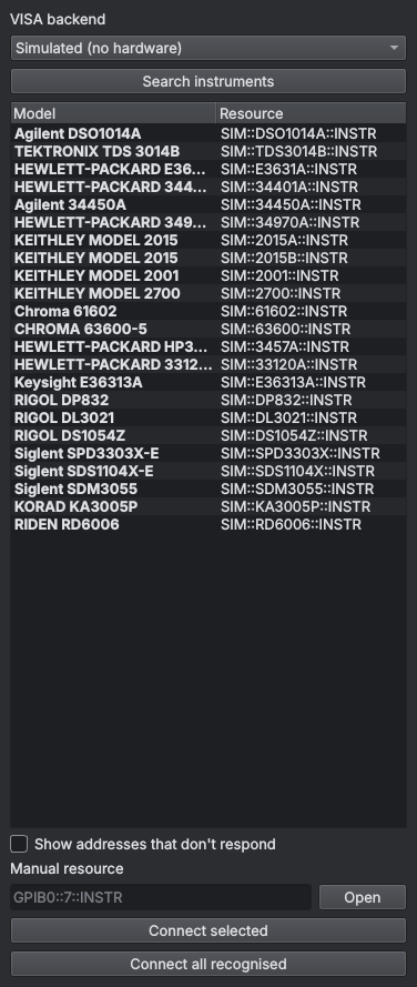
- Choose the VISA backend:
- Keysight IO Libraries: the normal choice. GPIB (82357B), USB and LAN. It also looks for USB instruments using the WinUSB driver (see code 48).
- pyvisa-py: without Keysight drivers (USB with WinUSB/libusb, LAN, serial).
- Simulated: no hardware.
- Press Search instruments. An Interface Clear is sent to the GPIB bus first to free it. Each instrument gets a few seconds to answer; the same button cancels the search.
- Double-click an instrument (or select several and press Connect selected). Connect all recognised opens every instrument that has a panel.
USB plug and play
Every 3 seconds OSA Lab checks whether a USB instrument has been plugged in or removed, without touching the GPIB bus. New ones appear in the list by themselves; unplugged ones (if not open) disappear. For GPIB press Search.
Addresses that don't respond
Keysight VISA lists the GPIB addresses saved in Connection Expert even if the instrument is off. OSA Lab hides them and the status bar says which. Tick Show addresses that don't respond to see them.
Manual resource
Type a VISA address (e.g. GPIB0::7::INSTR or TCPIP0::192.168.1.50::inst0::INSTR) and press Open.
Prologix and AR488 GPIB adapters
Prologix GPIB-USB, GPIB-ETHERNET and AR488 (Arduino) adapters do not use VISA: Instruments →
Prologix / AR488 GPIB adapters. Add the adapter (COM port or IP), press Test adapter and
Search addresses (tries *IDN? and ID? from 1 to 30) and save. With F5 they appear
as PROLOGIX::COM5::12::INSTR and work like any other GPIB instrument (several instruments on the same adapter share the
connection). Those that do not identify themselves are typed by hand in «GPIB addresses». An 82357B and one or more Prologix/AR488
can be used at the same time.
Serial port (RS-232 or USB-serial adapter)
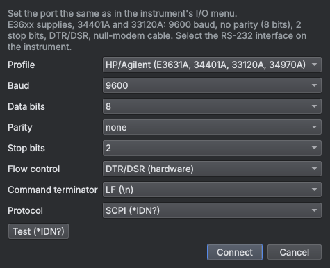
COM ports show up as Serial port COMn. Double-click to configure it: choose a profile (HP/Agilent: 9600 baud, 8 bits, no parity, 2 stop bits, DTR/DSR; Keithley: 9600 8N1, CR terminator…), press Test (*IDN?) and then Connect. The settings are saved for that port, so next time the instrument identifies itself. Right-click → Configure serial port… to change them.
Korad/Tenma and Riden supplies don't speak SCPI: choose their profile (or the matching Protocol) and OSA Lab
treats them like any other supply. Owon XDM meters use the "Owon XDM (115200 8N1)" profile.
The Fluke 8808A uses its own profile ("Fluke 8808A / 45"): it echoes and replies with the prompts => (OK),
?> (invalid command) and !> (cannot execute now), which OSA Lab handles. The Hioki instruments have their own
profiles (3157: CR LF and RTS/CTS; 3332: LF; set the 3332 to Co. mode, not Pr.). The 66xxB/C also have RS-232
(66xxA are GPIB only).
5. Workspace
- Each instrument opens as a window inside the workspace. Window menu: Tile, Cascade or Tabbed view.
- Another monitor: the ⧉ Detach to separate window button (top right of each window) or Ctrl+D. ⇲ Back to workspace brings it back.
- Save: File → Save workspace… stores instruments, positions, detached windows, panel settings, readings panels and the sequence. It is also saved automatically on exit and restored with Open last workspace.
- Closing an instrument window disconnects it and hands control back to its front panel (Local).
6. Plot and statistics
Almost every panel has a trend plot with its toolbar:
| Control | What it does |
|---|---|
| Window | Visible time: All, 30 s, 2 min, 10 min, 1 h. |
| Unit | Draws only the series in that unit (one consistent Y axis) or All. |
| Y axis | Auto (follows the reading), Auto from 0 or Manual (fixed minimum and maximum, e.g. 0–150 °C). |
| Freeze | Stops the plot while logging continues. |
| ● Log CSV | Writes every reading to a CSV in the data folder. |
| Cursors | Two draggable vertical lines: value of each series at C1 and C2, difference, mean between them and slope per minute (drift). Freezes the plot. |
| Compare… | Overlays the same readings from a recorded session (dashed line, aligned at the start): before/after a change. |
| Export / PNG / Clear | Saves everything collected as CSV, the plot as an image, or starts over. |
Below it, the statistics table: last value, minimum, maximum, mean, σ and number of readings. Tick or untick a series to show or hide it. Drag a column border to widen it; the width is remembered.
7. Saving the data
You don't need to remember anything: with File → Record the session automatically (on by default)
every reading from every instrument in Live, the calculated channels and the scope measurements are written to disk as they arrive,
in OSALab\sesiones\sesion_YYYYMMDD_HHMMSS.csv. Even if the program closes or the power goes, what was read is kept.
The status bar (bottom right) shows ● Recording session · N readings.
- File → Export session (Excel / CSV)… (Ctrl+E): choose the session (current or an earlier one), the format —Excel with one sheet per instrument or one CSV per instrument— and optionally just a time interval. Each reading is a column, with its label and unit.
- Start a new session closes the current file (e.g. when you change test); Open sessions folder to see or delete them.
- If you turn automatic recording off and exit with unsaved readings, the program asks whether to save them.
- Each plot's options (Export, ● Log CSV), the combined log and the sequence CSV/PDF are still available.
8. Custom labels
You can give each instrument and each reading your own name, e.g. Supply 1 for the E36313A and Output 1 voltage
for its CH1 6V V. The label shows up everywhere: window title, readings-panel tiles, plot legend and table, combined
log, sequencer and CSV headers (next to the original name).
- Reading: double-click (or right-click → Set label…) in the statistics table, in the combined log list, or right-click a tile → Label this reading….
- Instrument: Instruments → Name the active instrument… (F2), right-click in the instrument list, or on a tile → Name this instrument….
- Leave the text empty to go back to the original name.
- Labels are saved with the workspace and come back when you open it.
9. DC supply
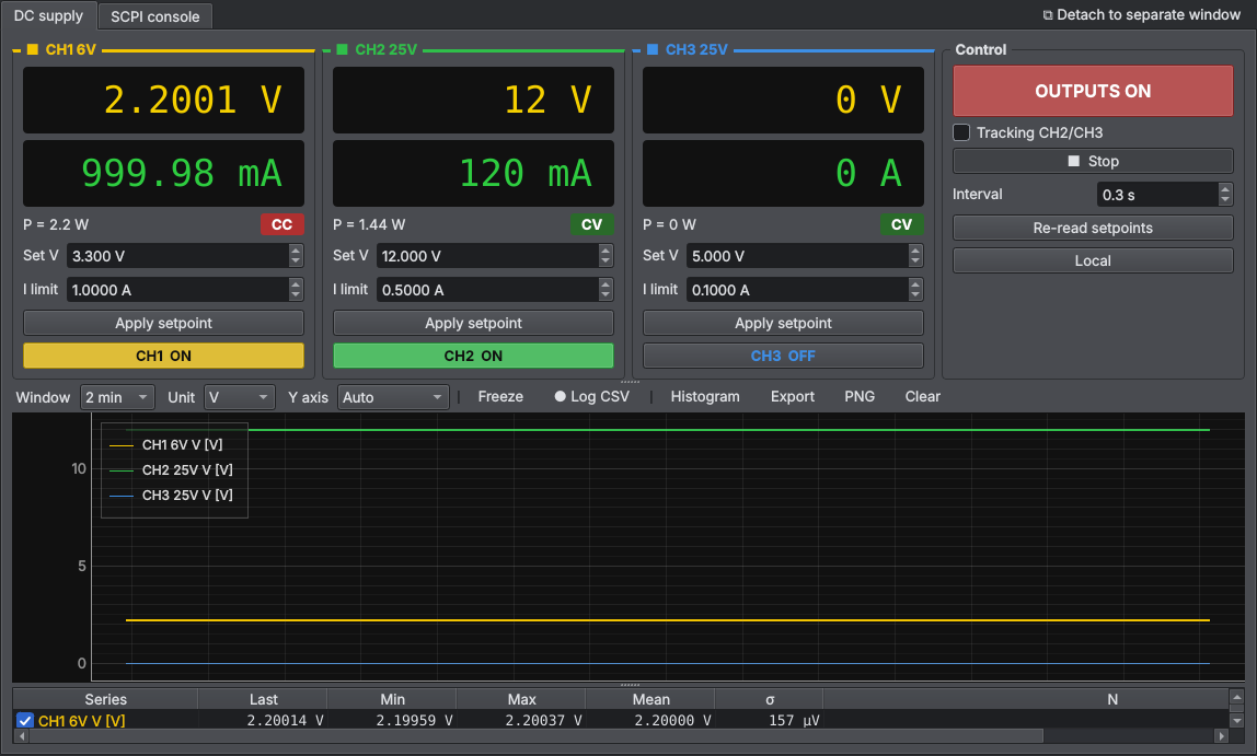
- Each output has its card: measured voltage and current, power, CV/CC indicator, voltage setpoint and current limit. Apply setpoint sends it.
- On the E36300 each channel has its own ON/OFF button; the big OUTPUTS button switches them all.
- Tracking: CH2/CH3 (E36300) or ±25 V (E3631A).
- ▶ Live reads periodically at the chosen Interval. Re-read setpoints refreshes the screen if you changed the supply by hand. Local hands control back to the front panel.
10. Multimeter
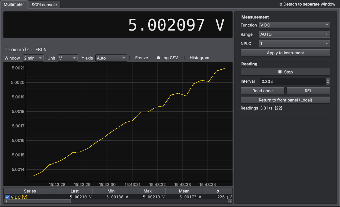
- Choose Function, Range and NPLC (speed/resolution) and press Apply to instrument.
- ▶ Live reads continuously, Read once takes a single reading, REL gives relative readings.
- Return to front panel (Local) releases the meter without closing the window.
- Keithley 2015/2016 THD: Distortion group (THD, THD+N, SINAD, number of harmonics, A, C, CCIR… filters) and Internal generator.
- Keithley meters are set to continuous trigger, so the instrument's display keeps working while you read.
11. Oscilloscope
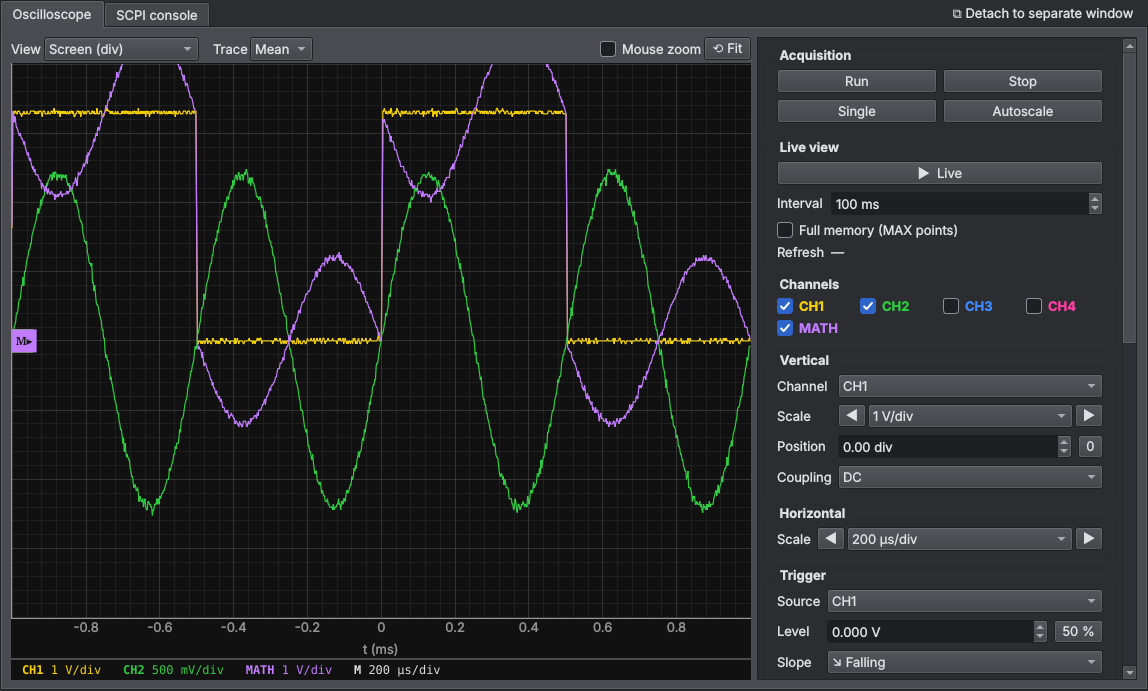
- View: Screen (div) draws each channel with its own position and scale, like on the scope; Volts puts every trace in real volts on the same axis.
- Trace: Mean (clean, like the screen) or Peak (keeps glitches and noise).
- Mouse zoom off: the plot always frames the screen. Turn it on to zoom with the wheel; ⟲ Fit returns to the full view.
- Acquisition: Run, Stop, Single, Autoscale. Live view: Live with its interval and Full memory (more points, slower).
- Channels: enable CH1–CH4 and MATH (FFT too, drawn separately against frequency).
- Vertical / Horizontal / Trigger: 1-2-5 knobs with ◀ ▶ like the scope's, position, coupling, source, level (50 %), slope and mode. Changes are sent immediately.
- Measurements: tick the ones you want (Vpp, frequency, Vrms…) per channel; they can be logged to CSV.
- Capture / export: Capture (in STOP, full memory), Save CSV, Save PNG, Scope screen (the instrument's own screenshot) and Cursors.
12. Data acquisition (34970A / Keithley 2700)
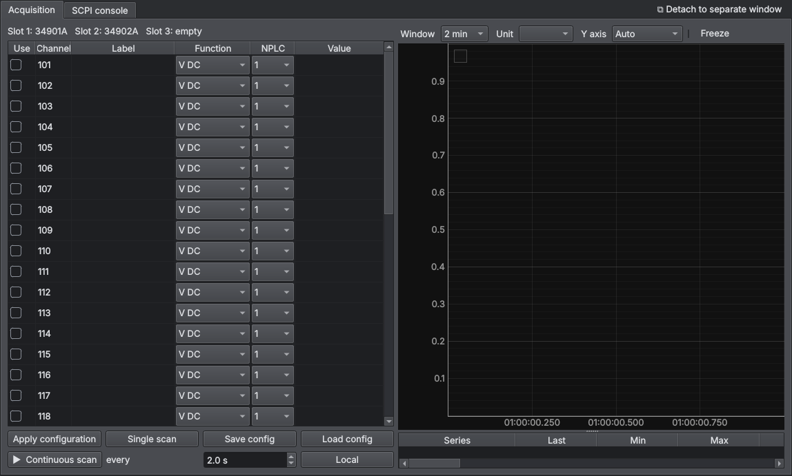
- On connection the installed cards and their channels are detected.
- Tick Use on the channels you want, give them a Label (e.g. Transformer) and choose the Function (V DC, K/J/T thermocouple, Pt100, NTC, Ω, I…) and NPLC.
- Apply configuration, then Single scan or ▶ Continuous scan with its interval.
- Save config / Load config store the channel table as JSON.
The Keithley 2700 also has a Multimeter (front) tab for the front terminals. Front and cards share the same internal DMM, so they are never both in Live at the same time.
13. Electronic load (Chroma 63600)
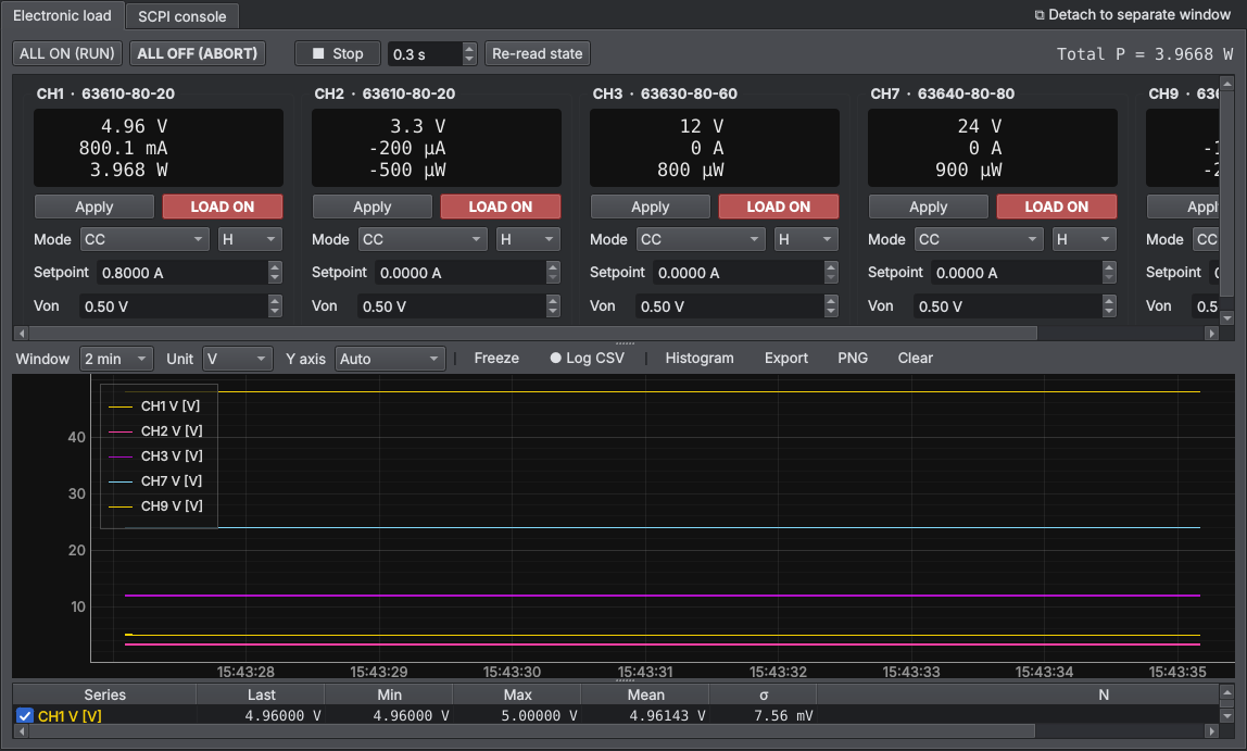
- Each channel: mode (CC, CR, CV, CP or dynamic CC), range (L/M/H or Auto), setpoint and turn-on voltage Von. Apply sends it and LOAD connects that channel.
- Dynamic CC: two levels, times and slew rates.
- ALL ON (RUN) / ALL OFF (ABORT) act on every channel; total power is shown at the top.
14. AC source (Chroma 61600)
- Setpoint: AC voltage, frequency, DC offset, range, coupling mode (AC/DC/AC+DC) and current limit.
- With Confirm when switching on ticked, it asks before enabling the output.
- Measurements: voltage, current, power, power factor, frequency and whatever else the model supports (discovered automatically and remembered per model and firmware). With the output OFF many measurements are not available.
15. Function generator
- Shape, frequency (accepts prefixes:
1k,2.5M,100m), amplitude (Vpp, Vrms or dBm), offset, duty cycle and the load the generator expects (50 Ω or High Z: it changes the real amplitude at the terminals). - The preview shows the ideal setpoint (it is not a measurement).
- Linear or logarithmic frequency sweep. The 33120A has no command to switch its output off: it is always on.
FFT analyzer (35670A)
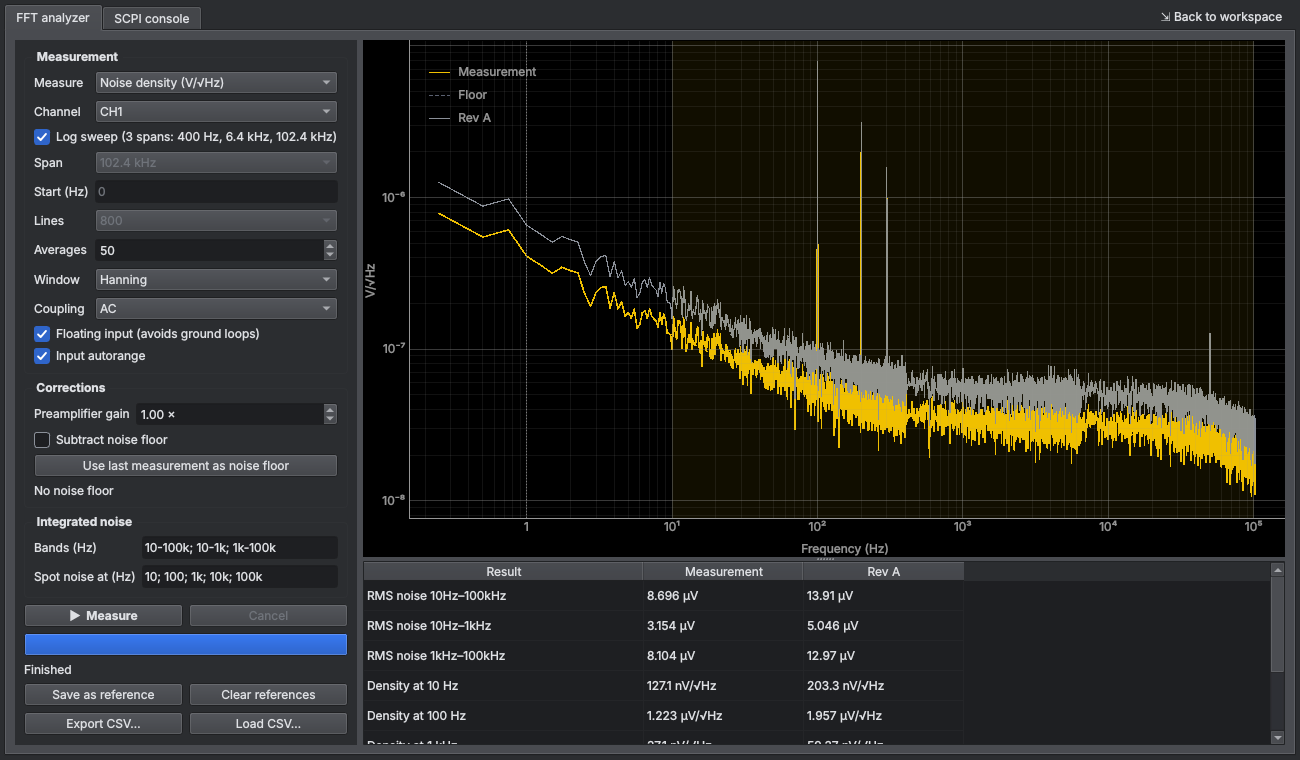
Measures noise spectral density (V/√Hz) or the spectrum (Vrms per line). With Log sweep it measures three 1600-line spans
(400 Hz, 6.4 kHz and 102.4 kHz) and joins them: 0.25 Hz resolution at the bottom and up to 102 kHz at the top. It gives the integrated RMS noise
over the bands you type (e.g. 10-100k; 10-1k; 1k-100k) and the spot noise at the frequencies you choose. It takes a preamplifier gain
(divided out) and subtracts the instrument's own noise floor (measured with the input shorted) in quadrature. Curves can be kept as references
or saved to CSV for comparison. With two identical preamplifiers (one per channel), Cross-correlation CH1×CH2 mode averages the cross spectrum: each preamplifier's own noise cancels out and the supply's noise remains; the dashed red curve is the limit reached with those averages. The two-channel preamplifier is in hardware/LNA_2CH (Fusion 360 project). Results are published as readings. How to set the measurement up: see the
power supply characterization guide.
66xx and E364x supplies
- HP/Agilent 66xx (6632B, 6652A…): one output; besides V and I, the panel logs whether it is in CC or CV and whether a protection (OV/OC) has tripped.
- E3640A–E3645A: one output with two ranges (e.g. E3644A 8 V/8 A and 20 V/4 A). The range is chosen automatically: if the requested voltage fits the low range, low is used (more current); otherwise high, with current limited to that range's maximum.
Network analyzer (8711/8712/8713/8714)
Parameter (S11, S21; S12 and S22 on ES models), start and stop frequency (accepts 300k, 10M, 1.3G), points,
IF bandwidth, power and averaging. Sweep makes a single sweep and Continuous repeats. The analyzer
sends the complex data already corrected by its calibration, and the panel computes the formats: dB magnitude, phase, unwrapped phase,
group delay, SWR, linear magnitude, R + jX impedance and the Smith chart.
- Markers: click on the plot (up to 4), draggable; maximum, minimum and −3 dB buttons (bandwidth, centre frequency and Q of a filter or resonator). The table gives frequency, value, impedance and difference from M1.
- Memory: stores the trace and shows data and memory, or data/memory (normalization, e.g. to remove a cable).
- Export: Touchstone
.s1p, or.s2pafter Measure S11, S21, S12, S22; and CSV.
Calibration is done on the analyzer itself (OSA Lab uses the corrected data).
Power meter (Hioki 3332)
Voltage, current, active, apparent and reactive power, power factor, phase angle, frequency and integration (Ah, Wh), in large tiles and on the plot. V and I ranges (or AUTO), rectifier mode (RMS, MEAN, MEAN + filter) and integration (start, stop, reset). Useful for the efficiency and no-load power of a supply: pick its "Active power" as the input power in Characterize power supply.
Ground bond (Hioki 3157)
Test current (3–31 A), upper and lower limits (in mΩ, up to 2 Ω) and time. START sends the settings and starts the test; the result is shown large (PASS / FAIL) with the measured resistance, and is kept in a history with the serial number of the device under test, exportable to CSV. Each result is published as a reading.
16. SCPI console
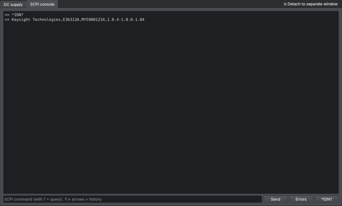
Each instrument has a SCPI console tab to send commands directly. If the command ends with
? the answer is read back. ↑ ↓ browse the history. Errors empties
the instrument's error queue and Diagnostics (on some instruments) tests which queries it answers.
17. Readings panel
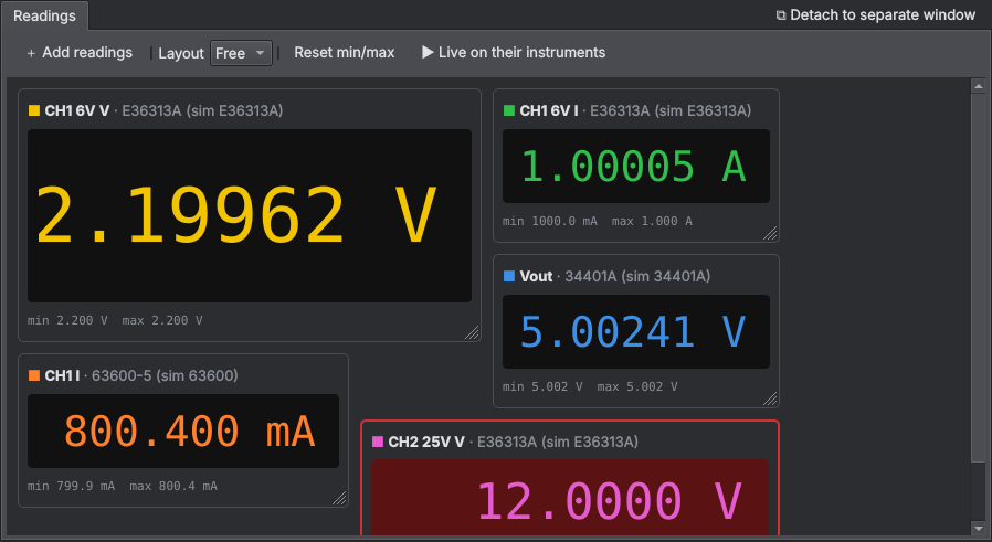
Tools → New readings panel (Ctrl+L). Shows the readings you choose, from any instrument, as big tiles in a single window. You can have several panels and move them to another monitor.
- Put the instruments in Live (or use ▶ Live on their instruments).
- + Add readings and pick one or more from the list.
- Right-click a tile for: label, colour, significant digits, limits (the tile turns red if the reading goes out of range), reset min/max or remove.
Layout
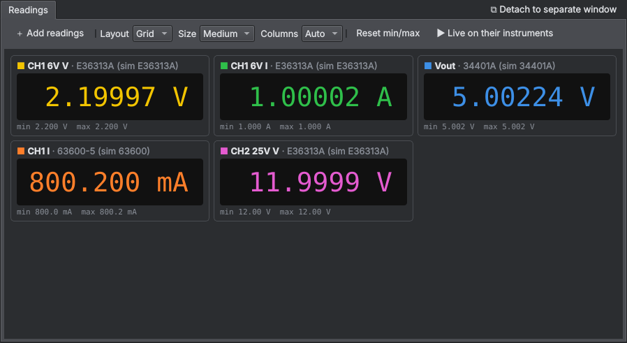
- Grid: tiles place themselves. Choose size and columns; drag a tile to reorder it.
- Free: drag each tile anywhere and resize it from the bottom-right corner; the number grows with the tile. Tiles snap to a 10 px grid (hold Alt for no snapping) and can overlap (Bring to front / Send to back).
If a tile stops receiving readings it turns grey and says for how long. The panel only displays: it never talks to the instruments.
18. Combined log
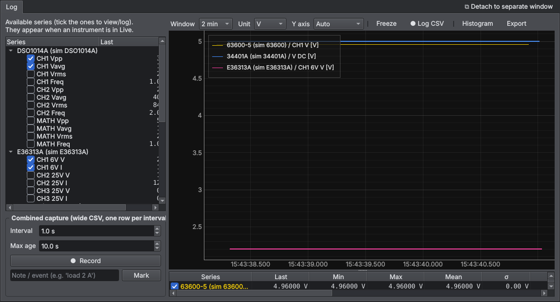
Puts readings from different instruments on one plot and into a single wide CSV (one row per interval, one column per series). Tick the series in the list on the left (they appear when the instrument is in Live), choose the Interval and press ● Record. Max age: if a series has no recent reading, its cell is left empty. Type a note and press Mark to leave an event mark in the CSV (e.g. "load 2 A").
19. Test sequencer
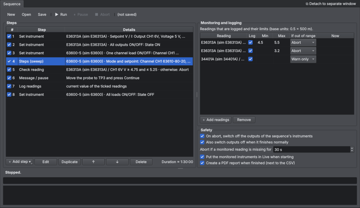
Tools → Test sequencer (Ctrl+T). Automates long tests: sets instruments, waits, checks and logs, while watching limits all the time.
Step types
| Step | What it does |
|---|---|
| Set instrument | DC supply (setpoint, outputs), load (mode and setpoint, ON/OFF), AC source, generator or a free SCPI command to any instrument. |
| Wait / hold | Waits a time (s, min, h) and optionally logs mean/min/max over that interval. |
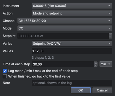
| Steps (sweep) | Repeats a setting with several values (1 ; 2 ; 3 or 0.5:0.5:3), holding each one for a time and logging at the end. |
| Log readings | Saves a row with the current values. |
| Check reading | Checks that a reading is between minimum and maximum; if not, aborts or logs FAIL and continues. |
| Message / pause | Stops until you press Continue (e.g. to move a probe). |
| Ramp (over time) | Moves a setpoint from one value to another over a time (e.g. supply 0→12 V in 2 s, or load 0→5 A in 10 min), updating every N s. |
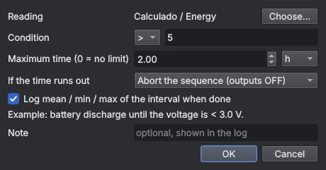
| Wait until… | Waits until a reading (or a calculated channel) is above or below a value, with a maximum time. E.g. battery discharge until < 3.0 V. |
Example: load step test
- Connect the supply, the load and the instrument measuring temperatures, and put them in Live.
- Steps: Set supply to 5 V → Set outputs ON → Set load ON →
Steps on the load (CC, values
1 ; 2 ; 3, 30 min each) → Set loads OFF. - In Monitoring and logging, + Add readings: output voltage, current, temperatures.
Give them a minimum/maximum (in base units:
0.5= 500 m) and choose Abort or Warn only. - ▶ Run. The bar shows the step, the time left and the total.
Safety
- If a monitored reading goes out of its limit (with action Abort), the sequence stops and switches off the outputs of the instruments it controls (supplies, loads, AC source, generator).
- If a monitored reading stops arriving for the configured time (hung instrument, Live stopped), it aborts too.
- ⏸ Pause freezes the timer but keeps watching limits; ■ Abort stops and switches off.
- Commands run in a separate thread: the window never freezes.
Example: battery test
- In Tools → Calculated channels create "Charge Ah = ∫ I dt" with the load current.
- Steps: Set load CC 1 A → Set load ON → Wait until battery voltage < 3.0 V (max 10 h) → Set load OFF → Log readings.
- Monitor voltage, current, the Ah channel and temperature (with a safety limit).
Results
Each run creates secuencias/<name>_<date>.csv in the data folder (; separator, opens
directly in Excel): one row per setting and per logged point, with mean, minimum and maximum of every reading. Sequences
are saved as .seq.json and also with the workspace.
With Create a PDF report when finished a PDF report is also created next to the CSV: result, steps, limits, plots of the logged readings and the results table (red rows = failures or abort). If notifications are set up, you get a message when it finishes or aborts.
20. Analysis tools
In the Tools menu.
Bode plot
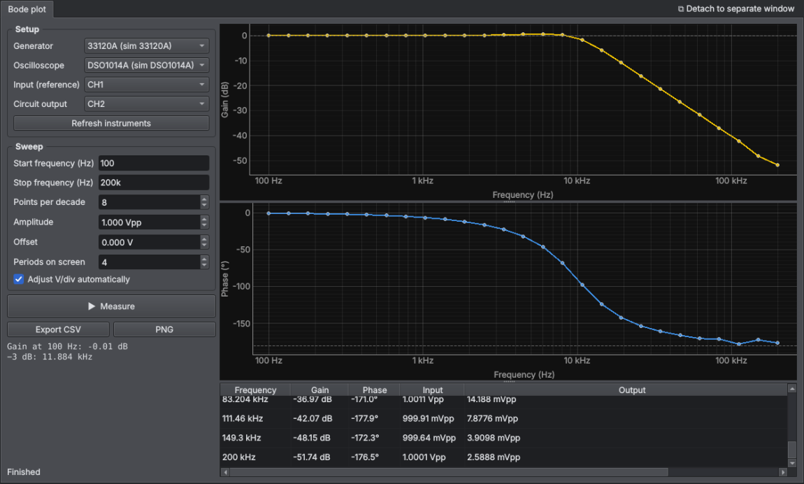
Measures the frequency response of a circuit with any supported generator and oscilloscope (Ctrl+B, or the button on the scope panel).
- Connect the generator to the circuit input and feed that same signal to a scope channel (reference, e.g. CH1). The circuit output goes to another channel (e.g. CH2).
- Choose start and stop frequencies (
k,Maccepted), points per decade and amplitude. - ▶ Measure. At each frequency the timebase and, if ticked, each channel's V/div are adjusted. Amplitude and phase are computed by fitting a sine to each trace, so noise barely matters.
When done it shows the low-frequency gain, the −3 dB frequency and, if 0 dB or −180° are crossed, the phase and gain margins (useful for regulator loop stability). Export CSV and PNG.
Calculated channels
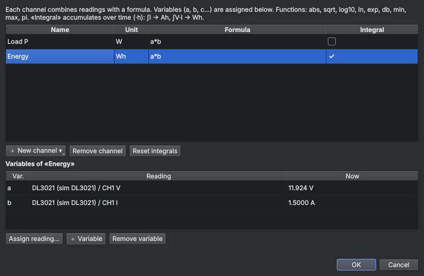
Formulas with readings from any instrument (Ctrl+K): power a*b, efficiency
100*(a*b)/(c*d), ΔT a-b, gain db(a/b)… Each letter is assigned to a reading. With
Integral it accumulates over time in hours: ∫ I → Ah, ∫ V·I → Wh (Reset integrals
to start again). The result appears as the "Calculated" instrument: it can go on tiles, the combined log, the XY plot and the
sequencer, with limits. Saved with the workspace.
XY plot
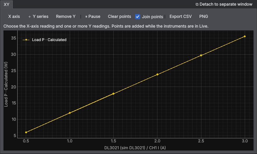
One reading against another: efficiency versus current, Vout versus Vin… X axis… and + Y series…; each new Y reading is plotted with the latest X value. Export to CSV or PNG.
Histogram
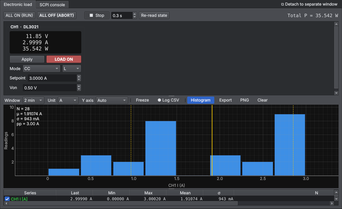
On any plot, the Histogram button shows the distribution of the series selected in the table, with mean, σ and peak-to-peak: useful to see a measurement's noise and stability.
Live oscilloscope screen
Live screen button on the scope panel: a copy of the instrument's own screen that refreshes by itself (adjustable rate), with a button to save the image.
Arbitrary waveform
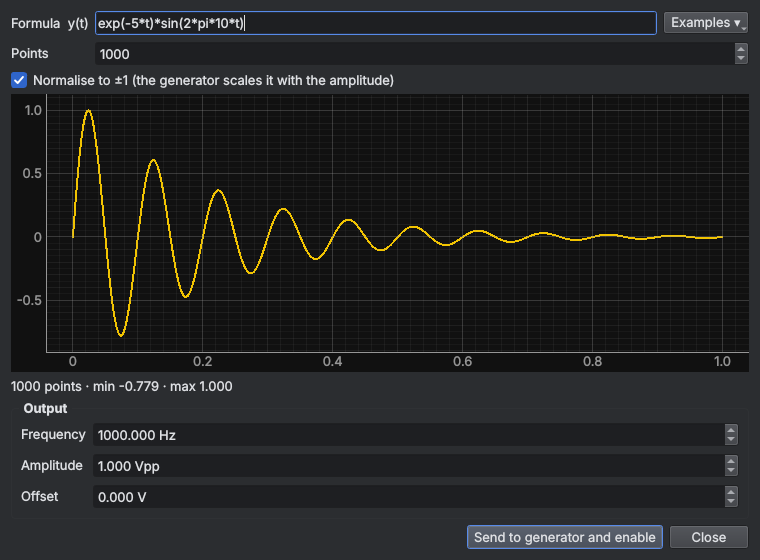
Arbitrary waveform… button on the generator: type a formula in t (0 to 1 = one period),
pick an example or import a CSV, check the preview and press Send to generator and enable.
Python console
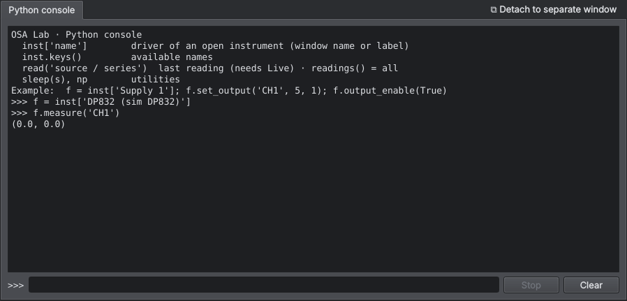
To write your own scripts with the instruments already open (Ctrl+Shift+P):
inst['Supply 1'] gives the driver (by window name or label), read('source / series') the last reading.
Each command runs in its own thread; Stop interrupts it.
Notifications (sound, Telegram, e-mail)
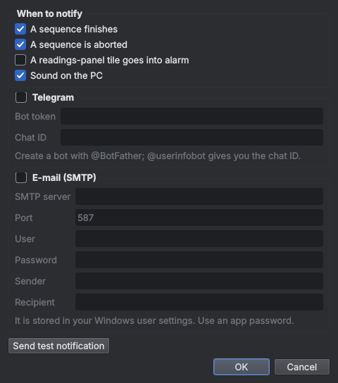
To find out away from the bench when a sequence finishes or aborts, or a tile goes into alarm. Telegram: create a bot with @BotFather, paste its token and your chat ID. E-mail: SMTP server with an app password. Send test notification to check.
Characterize power supply
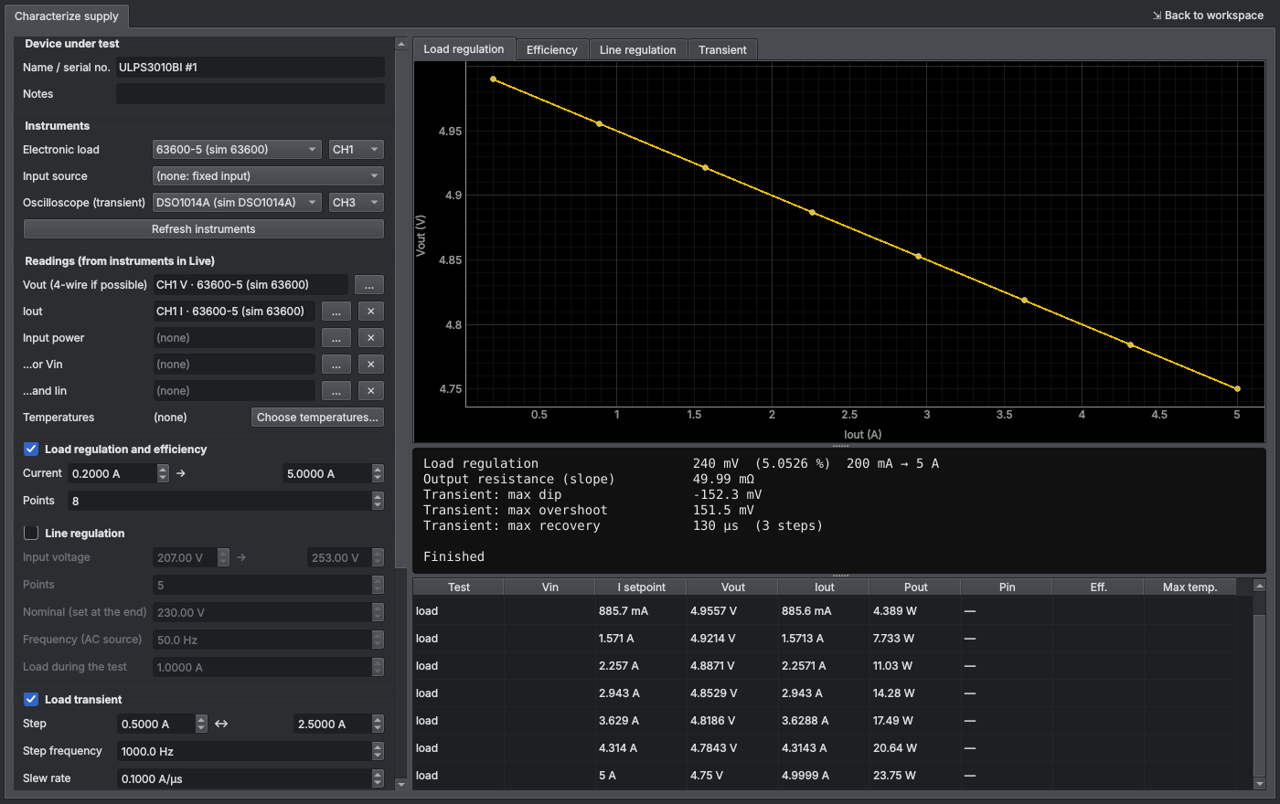
Tools → Characterize power supply (Ctrl+Shift+C). A wizard that, with the electronic load, the input source and the oscilloscope, runs:
- Load regulation and efficiency: current sweep; Vout, Pout, efficiency, output resistance and temperatures at each point.
- Line regulation: input voltage sweep (AC or DC source) at fixed load; goes back to nominal at the end.
- Load transient: load in dynamic mode L1↔L2 with a fixed slew rate and scope in AC; maximum dip/overshoot and recovery to a band.
Readings (Vout, Iout, input power, temperatures) are chosen from the instruments in Live, so any multimeter or acquisition channel works.
Safety limits (minimum Vout, maximum temperature), and the load is turned off at the end or on stop. It creates a CSV and a PDF report
in OSALab\caracterizacion. Help → Guide: characterizing power supplies explains each measurement, the setup and
which instrument to use.
Ripple and noise with the oscilloscope
Tools → Ripple and noise with the oscilloscope (Ctrl+Shift+R). Sets the channel to AC and 20 MHz, the preset timebase (100 Hz mains, switching, spikes), takes N captures and gives the worst peak-to-peak, the mean RMS and the main spectral tones (Hann-window FFT). Reference for comparison and CSV export.
Protections (interlocks)
Tools → Protections. Rules that always watch the readings, with or without a sequence: "heatsink T > 85 °C for 2 s", "Vout < 4.5 V", or "reading stops arriving for more than 30 s". Action: turn off all outputs (supplies, loads, AC source and generators), stop the sequence, or notify only; it always notifies (sound, Telegram, e-mail). The status bar shows how many are active. They are saved with the workspace. The manual stop for everything is Instruments → STOP (Ctrl+Shift+X).
Remote control from phone
Tools → Remote control from phone. Starts a small web server on the local network: from the phone's browser (same Wi-Fi) you see all readings live, and a STOP button turns off all outputs. PIN protected; it does not go out to the Internet. The first time, Windows asks about the firewall: allow private networks only.
Instrument explorer (new driver)
For instruments without a driver. Connect it (it opens with the SCPI console), then in Tools → Instrument explorer press
Probe commands: it sends typical SCPI queries for each family (queries only, nothing is changed) and records which ones answer. Then
Generate driver writes a Python draft with the right base class and the commands that worked; it is saved in
OSALab\drivers_nuevos to review and add (see CONTRIBUTING.md).
Certification tests (CE / UL)
Tools → Certification tests (CE / UL) (Ctrl+Shift+E). Safety and EMC pre-compliance testing of power supplies to IEC/EN/UL 62368-1, 61010-1, 60335-1 or 60601-1:
- Fill in the equipment data (rated voltages, current and power, class I/II, circuit protection, maximum ambient temperature…), choose the standard and press Generate the test plan.
- Each test has four tabs: Connection and procedure (diagram of where each lead goes), Parameters and limits (editable), Run (choose the instruments and start) and Result (table, PASS/FAIL, remarks and photos).
- Automatic: AC/DC hipot, insulation, ground bond and touch/leakage current with the Omnia (or ground bond with the Hioki 3157); input with AC source + power meter; heating with thermocouples until steady state and correction to the maximum ambient; simulated faults (power and temperature log); conducted emissions with LISN and spectrum analyzer, with the CISPR limits drawn (with an E7401A–E7405A, doubtful peaks are measured automatically with quasi-peak and average); current harmonics (EN 61000-3-2, oscilloscope with current probe) and external power supply ecodesign (EU 2019/1782: average efficiency and no-load power).
- Before each high-voltage or high-current test it asks you to confirm the safety conditions.
- Save stores the project (
.osacert, inOSALab\certificacion) and PDF report creates the report with the diagrams, parameters, measurements, instruments and calibrations.
HP 3585A. It does not answer *IDN?: in the instrument list, right-click its GPIB address (11 from the factory;
enable "Show addresses that do not answer") → Assign model… → HP 3585A. Set it up on the front panel (START 150 kHz,
STOP 30 MHz, RBW 30 kHz, dB scale, 50 Ω input); OSA Lab reads the settings from the screen text and trace A.
It is a pre-compliance test: values are typical ones and those marked "verify" depend on tables in the standard. How to connect each test, which equipment is needed and the values of each standard are in the certification test guide.
Production test bench
Tools → Production test bench (Ctrl+Shift+F). End-of-line test for series production:
- Create the product profile: input voltage, instruments and steps with their parameters and limits (double-click the cell; JSON format,
e.g.
{"lo": 29.7, "hi": 30.3}). Available steps: ground bond and hipot (Omnia or Hioki 3157), no-load consumption, output voltage at a given current, load regulation, ripple and noise (oscilloscope, AC + 20 MHz), efficiency and overcurrent protection trip point. Save it as.osaprod. - Type or scan the serial number and press Enter (a barcode reader works). PASS/FAIL appears in large letters with the detail of each step.
- Each unit is stored in
OSALab\produccion\produccion.db(SQLite) and its PDF certificate is created with the measurements and the instruments used, with their calibration date from the inventory. Optional: 62 × 29 mm label with QR for units that pass. - Below: today's units, first-pass yield, history, open certificates and export the history to CSV (one column per measurement).
It warns you if a serial number is repeated. At the end it turns off the load and, optionally, the AC source. The safety steps use the same code as the certification tests; the EUT must be able to switch from the AC source to the Omnia (relay fixture or a separate station).
Inventory and calibrations
Tools → Inventory and calibrations (Ctrl+Shift+I). List of your instruments
with serial number, last calibration, due date, laboratory, certificate number and file. Add the connected instruments fills them in
from *IDN?. Connecting an instrument whose calibration has expired shows a warning (and a status bar note if it expires within
30 days). Certification reports and production certificates take the calibration date from here. CSV import and export.
Telemetry from your boards over a serial port
Connect your board's UART (or its USB-CDC) and, in the port settings, choose the My board's telemetry profile (115200 8N1, LF). Every line the firmware sends becomes readings, like those of an instrument: plot, log, session, protections and sequencer.
- key=value (automatic):
vbus=3.301V iload=12.5mA tmcu=24.5°C state=2. Prefixed units are converted (12.5mA → 0.0125 A). Alsovbus[V]=3.3orkey: value. - CSV:
3.301,12.5,24.5; names come from a header line or from the "CSV columns" field. - JSON per line or a regular expression with named groups.
- Lines without numbers (log messages) are shown below and produce no readings. "Send to the firmware" sends a command over the UART.
Battery test
Tools → Battery test (Ctrl+Shift+A). Choose the chemistry (Li-ion, LiFePO4, NiMH, lead-acid), the cells in series and the capacity: the cut-off and charge voltages and the currents are proposed (C/5 discharge, C/2 charge, end at C/50).
- Discharge with the electronic load in CC, CR or CP down to the cut-off voltage: capacity in mAh and Wh, average voltage and, in CC, internal resistance from current pulses (ΔV/ΔI) every few minutes.
- CC/CV charge with a power supply until the current drops below the end value. It asks for confirmation: a wrongly configured charge can set the battery on fire.
- Optional: a temperature reading (thermocouple on the battery) that stops the test if it exceeds the maximum.
- Plots of voltage versus capacity, versus time and of internal resistance; automatic CSV in
OSALab\bateriasand PDF report.
Efficiency map (Vin × load)
Measurements → Efficiency map (Ctrl+Shift+M). With a power supply on the converter input and the
electronic load on its output, it steps through a list of input voltages and, for each, a list of load currents. At every point it
reads Vin·Iin from the supply (or Iin with a multimeter) and Vout·Iout from the load and computes η. Result: a heat map of
efficiency, losses, Vout or Pin; η–Iout curves per Vin; a table; load and line regulation, and CSV/PNG. Lists: 5, 12, 24,
0:0.25:2 (start:step:stop) or 0.1-2/8 (8 points). «Minimum Vout» moves on to the next Vin if the converter drops out.
PSRR and output noise
Measurements → PSRR and output noise (Ctrl+Shift+Y). PSRR: the generator injects a sine at the regulator input through an injector (Picotest J2120A, transformer or MOSFET stage on the DC rail); the scope measures the regulator input (at its pins) and the output, both AC-coupled. At each frequency a sine is fitted to each trace and N captures are averaged coherently (noise drops by √N); vertical scales are set automatically. PSRR = 20·log(Vin/Vout) + the gain of the preamplifier on the output, if any. Points where the output is below the measurement noise are marked «≥»: the regulator is at least that good. Reference curve loads the datasheet curve (CSV frequency;dB) for comparison.
Output noise: density in V/√Hz with the scope (Welch with Hann window over the full memory, several captures) or with the 35670A FFT analyzer. A low-noise LDO (a few µVrms) needs a 40–60 dB low-noise preamplifier and a clean supply for the setup; Measure floor with the preamplifier input shorted and it is subtracted. It gives the integrated noise in the chosen band (10 Hz–100 kHz, as manufacturers do) and the density at 10 Hz, 100 Hz, 1 kHz, 10 kHz and 100 kHz.
Characterization report
Tests → Characterization report (Ctrl+Shift+G) gathers in a PDF (or HTML) with your header the results of the open tools: characterize supply, efficiency map, ripple, PSRR, noise, Bode and I-V curves. It starts with a summary of all quantities, continues with one section per test (white-background plots and tables) and ends with the list of instruments with manufacturer, model, serial number and calibration date from the inventory. Fill in the equipment, serial number, customer and reference; To notebook copies the sections into the lab notebook to keep annotating.
Sequence templates
Tests → Sequence templates: ready-made bench sequences (DC-DC start-up and regulation, line regulation, burn-in
with monitoring, power cycling, battery discharge). When you choose one, you assign the open instruments to each role (supply, load and
their output or channel), the readings to monitor and the parameters (Vin, tolerance, duration…); it is loaded into the sequencer to
review and run. Save the current sequence as a template turns yours into a template (instruments become roles), in
OSALab\plantillas, to use on another bench or share.
I-V curves
Tools → I-V curves (Ctrl+Shift+V). Sweeps voltage (or current, with an SMU) and measures the current. Works with an SMU (Keithley 2400/2450, Keysight B29xx), with a lab supply (measuring with its readback or with a multimeter in current mode) or with the electronic load in CV for solar panels, cells and power supplies.
- Presets: diode/LED forward and reverse, zener, resistor, solar panel.
- Several overlaid curves (e.g. several LEDs), logarithmic |I|, power P = V·I, forward and back to see hysteresis.
- Automatic analysis: Vf at 1 and 10 mA, ideality factor n, Is, Rs, reverse leakage; R by linear fit; for panels, Pmax, Voc, Isc and fill factor.
Lab notebook
Tools → Lab notebook (Ctrl+Shift+N). Collects in order notes, captures of any window
(plots, panels, tools), the oscilloscope screen, a table with the current readings and images. It is saved as .osanote and exported
to PDF or HTML (single file) with your company header (name, logo, author).
Automation API
Tools → Automation API. Enables an HTTP/JSON server (this PC only by default, with a token) to control OSA Lab from
scripts: list instruments, read readings, send SCPI commands, call driver methods (set_output, measure,
apply…), connect, open workspaces and STOP. The Python client tools/osalab_client.py needs nothing else;
tools/test_ejemplo_api.py is a pytest example. OSALab.exe --api starts it even if it is not enabled.
User drivers (plugins)
At startup OSA Lab loads the .py files in OSALab\drivers: every class that inherits from an instrument type
(PowerSupply, Multimeter, ElectronicLoad, FunctionGenerator, SourceMeter…) and has
models is used with the standard panel of that type. The instrument explorer generates the draft and installs it with one button.
Help → User drivers shows the loaded ones and the errors, and creates an example template.
Languages
The interface is available in Spanish, English, German, French, Italian and Portuguese (View → Language; the manuals in Spanish and English). More languages can be added with a JSON file: Help → Translate OSA Lab into another language
creates the template in OSALab\i18n. Anything not translated is shown in English, so it can be done in parts.
Instruments that do not respond
Panel commands (outputs, setpoints, configure, SCPI console, safety tests, GPIB reset) run in the background and in the order you press them, with or without Live: if an instrument is off or hung, the window stays responsive and the error appears in the status bar when its timeout expires. Each GPIB bus (and each USB, LAN or serial instrument) has its own turn, so a hung instrument does not delay those on other buses or the STOP.
Modules and activation
OSA Lab starts with the base program: finding and operating instruments, readings panel, log, XY plot, calculated channels, SCPI console, sequencer and templates, STOP and protections, and inventory. Everything else is in modules that do not appear in the menus until they are activated in Help → Modules and activation with an OSA Electronics code:
| Module | Includes |
|---|---|
| Power supplies | Characterize supply, efficiency map, ripple and noise, PSRR and output noise, characterization report |
| Analysis | Bode plot and I-V curves |
| CE / UL certification | Safety, conducted EMC, harmonics and ecodesign pre-tests |
| Production | Production test bench |
| Batteries | Battery test |
| Automation | API, remote control from phone, Python console, instrument explorer, user drivers |
| Notebook and notifications | Lab notebook and notifications |
A code can activate one module, a pack (electronics bench: supplies, analysis and notebook; test laboratory: certification, production and batteries) or everything (master code). If the code is issued to you, type in «User» the name or e-mail it was issued to (case and accents do not matter). Trial codes expire on the date given and the module is hidden again. A workspace that uses a module that is not activated still opens, without that tool.
Request free trial… asks osalab.io for a 30-day trial of a module (or a pack, which is reviewed by hand): you receive an e-mail to confirm your address and then the code. Recover my codes… e-mails you all the active codes for your address. Once a day, when online, OSA Lab downloads the list of revoked codes (this can be turned off in Help → About → Updates). Without internet everything keeps working: codes are checked inside the program.
21. Menus and updates
| Menu | Contents |
|---|---|
| File | New / open / recent / save / save as workspace, session recording and export, data folder, exit. |
| Instruments | Search (F5), network search (LXI), Prologix/AR488 GPIB adapters, connect or disconnect all, Live on all, STOP (all outputs off), protections, instrument name, inventory and calibrations, reset GPIB, demo mode. |
| Measurements | Readings panel, combined log, XY plot, calculated channels · Bode, ripple and noise, I-V curves, PSRR and output noise · characterize supply, efficiency map. |
| Tests | Sequencer and sequence templates · certification tests, production bench, battery test · characterization report. |
| Tools | Lab notebook, notifications, remote control from phone, automation API · instrument explorer, user drivers, Python console · find a function (Ctrl+P). |
| View | Theme, font size, language, instrument list, status bar, full screen (F11). |
| Window | Tile, cascade, tabs, detach/attach, minimise, close, go to… |
| Help | Manual, power supply characterization guide, certification test guide, shortcuts, program log, data folder, check for updates, about. |
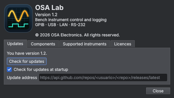
Help → About shows the version, the OSA Electronics copyright, the components used, the list of supported instruments and the licences. Check for updates queries osalab.io (stable or beta channel; GitHub releases or your own JSON also work) and, if there is a new version, shows what's new. If the release includes the installer, Download and install downloads it, checks its SHA-256 checksum (if published), closes OSA Lab saving the workspace, installs and reopens it. It can check automatically at startup (it only offers the update when no instruments are open).
Find a function (Ctrl+P, or the button on the quick access bar): type part of the name («bode», «stop», «battery», «template»…) and press Enter; it searches all menus. The quick access bar (Search, Network, Readings panel, Sequencer, Live all, Stop Live and STOP) can be hidden in View → Quick access bar.
22. Theme, font and language
- View → Dark theme / Light theme.
- View → Font size: Normal, +1, +2 or +3 points (menus included). Applied immediately.
- View → Language: Español or English. Asks to restart the program.
23. Files and folders
Everything is stored in the data folder %USERPROFILE%\OSALab (File → Open data folder):
*.csv | Plot logs, oscilloscope captures, combined log. |
sesiones\ | Automatic recording of every reading of each session. |
secuencias\ | Saved sequences and their results. |
*.osalab | Workspaces (JSON). With the installer, double-clicking opens OSA Lab with that workspace. |
caracterizacion\ | CSV and PDF reports from power supply characterization. |
drivers_nuevos\ | Driver drafts from the instrument explorer. |
ultimo_espacio.json | Last workspace (saved on exit). |
osalab.log | Program log (useful for diagnosing problems). |
cuelgue_*.txt | If the window blocks for more than 6 s, this records where it was waiting. |
24. Troubleshooting
No GPIB instrument responds
An instrument can leave the bus stuck mid-handshake. Use Instruments → Reset GPIB bus; if that doesn't help, power-cycle the last instrument you connected, or unplug and replug the 82357B.
A USB instrument doesn't appear, not even in Connection Expert (code 48)
Some Keysight/Agilent instruments (E36313A, 34405A…) use the ausbtmc USB-TMC driver, which Windows 11 may
block: Device Manager shows a yellow triangle and code 48. Fix:
- Download Zadig and enable Options → List All Devices.
- Pick the instrument by checking its USB ID (e.g. E36313A =
2A8D 1202, 34405A =0957 0618). Don't touch the 82357B (0957 0718). - Driver WinUSB → Replace Driver. OSA Lab detects it within seconds (Keysight backend).
To undo: Device Manager → the instrument → Uninstall device (ticking "delete the driver").
Windows detects nothing when plugging in a USB instrument
Try another cable (many are charge-only), another port without a hub, and check the instrument's USB mode (some scopes have Auto/Printer/Device: it must be Device).
Odd readings, or the Chroma gives no measurements
With the output OFF many AC sources return no measurements. Press Diagnostics in the SCPI console to see what it answers.
The window froze
Look at the latest cuelgue_*.txt and osalab.log in the data folder.
25. Keyboard shortcuts
| Ctrl+O | Open workspace |
| Ctrl+S | Save workspace |
| Ctrl+D | Detach the active window (other monitor) |
| Ctrl+L | New readings panel |
| Ctrl+T | Test sequencer |
| F2 | Name the active instrument |
| F5 | Search instruments |
| Ctrl+E | Export session |
| Ctrl+B | Bode plot |
| Ctrl+K | Calculated channels |
| Ctrl+Shift+C | Characterize supply |
| Ctrl+Shift+E | Certification tests |
| Ctrl+Shift+F | Production bench |
| Ctrl+Shift+I | Inventory and calibrations |
| Ctrl+Shift+A | Battery test |
| Ctrl+Shift+V | I-V curves |
| Ctrl+Shift+N | Lab notebook |
| Ctrl+Shift+L | Search on the network (LXI) |
| Ctrl+Shift+R | Ripple and noise with the oscilloscope |
| Ctrl+Shift+X | STOP: turn off all outputs |
| Ctrl+Shift+P | Python console |
| Ctrl+Shift+S | Save workspace as… |
| Ctrl+W | Close active window |
| F11 | Full screen |
| F1 | This manual |